How Far is Video Generation from World Model?
— A Physical Law Perspective
We conduct a systematic study to investigate whether video generation is able to learn physical laws from videos, leveraging data and model scaling.


We conduct a systematic study to investigate whether video generation is able to learn physical laws from videos, leveraging data and model scaling.


👉What? We study whether video generation model is able to learn and stick to physical laws.
👉Why?
OpenAI’s Sora
Scaling video generation models is a promising path towards building general purpose simulators of the physical world.
However, the ability of video generation models to discover such laws purely from visual data without human priors can be questioned. A world model learning the true law should give predictions robust to nuances and correctly extrapolate on unseen scenarios.
👉How? Answering such an question is non-trivial as it is hard to tell whether a law has been learned or not.
👉Key Messages
We aim to establish the framework and define the concept of physical laws discovery in the context of video generation.
In classical physics, laws are articulated through mathematical equations that predict future state and dynamics from initial conditions.
In the realm of video-based observations, each frame represents a moment in time, and the prediction of physical laws corresponds to
generating future frames conditioned on past states.
Consider a physical procedure which involves several latent variables $\boldsymbol{z}=(z_1,z_2,\ldots,z_k) \in \mathcal{Z} \subseteq \mathbb{R}^k$,
each standing for a certain physical parameter such as velocity or position. By classical mechanics, these latent variables will evolve by differential
equation $\dot{\boldsymbol{z}}=F(\boldsymbol{z})$. In discrete version, if time gap between two consecutive frames is $\delta$, then we have
$\boldsymbol{z}_{t+1} \approx \boldsymbol{z}_{t} + \delta F(\boldsymbol{z}_t)$. Denote rendering function as
$R(\cdot): \mathcal{Z}\mapsto \mathbb{R}^{3\times H \times W}$ which render the state of the world into an image of shape $H\times W$ with RGB channels.
Consider a video \( V = \{I_1, I_2, \ldots, I_L\} \) consisting of \( L \) frames that follows the classical mechanics dynamics. The physical coherence
requires that there exists a series of latent variables which satisfy following requirements:
$$ \boldsymbol{z}_{t+1} = \boldsymbol{z}_{t} + \delta F(\boldsymbol{z}_t), t=1,\ldots,L-1. $$
$$ I_t = R(\boldsymbol{z}_t), \quad t=1,\ldots, L. $$
We train a video generation model \( p \) parametried by \( \theta \), where \( p_{\theta}(I_1, I_2, \ldots, I_L )\) characterizes its understanding of
video frames. We can predict the subsequent frames by sampling from \( p_{\theta}(I_{c+1}', \ldots I_L' \mid I_1, \ldots, I_c) \) based on initial frames'
condition. The variable $c$ usually takes the value of 1 or 3 depends on tasks. Therefore, physical-coherence loss can be simply defined as
$-\log p_{\theta}(I_{c+1}, \ldots, I_L \mid I_1, \ldots, I_c) $. It measures how likely the predicted value will cater to the real world development.
The model must understand the underlying physical process to accurately forecast subsequent frames, which we can quantatively evaluate whether video
generation model correctly discover and simulate the physical laws.
Suppose we have a video generation model learned based on the above formulation. How do we determine if the underlying physical law has been discovered?
A well-established law describes the behaviour of the natural world, e.g., how objects move and interact. Therefore, a video model incorporating
true physical laws should be able to withstand experimental verification, producing reasonable predictions under any circumstances, which demonstrates
the model's generalization ability. To comprehensively evaluate this, we consider the following categorization of generalization
(see Figure 1) within the scope of this paper:

We focus on deterministic tasks governed by basic kinematic equations, as they allow clear definitions of ID/OOD and straightforward quantitative error evaluation.

In-Distribution (ID) Generalization. As in Figure 3, increasing the model size (DiT-S to DiT-L) or the data amount (30K to 3M) consistently decreases the velocity error across all three tasks, strongly evidencing the importance of scaling for ID generalization. Take the uniform motion task as an example: the DiT-S model has a velocity error of $0.022$ with 30K data, while DiT-L achieves an error of $0.012$ with 3M data, very close to the error of $0.010$ obtained with ground truth video.
Out-of-Distribution (OOD) Generalization. The results differ significantly.
We also trained DiT-XL on the uniform motion 3M dataset but observed no improvement in OOD generalization. As a result, we did not pursue training of DiT-XL on other scenarios or datasets constrained by resources. These findings suggest the inability of scaling to perform reasoning in OOD scenarios. The sharp difference between ID and OOD settings further motivates us to study the generalization mechanism of video generation in Section 4.1.
It is understandable that video generation models failed to reason in OOD scenarios, since it is very difficult for humans to derive precise physical laws from data. For example, it took scientists centuries to formulate Newton's three laws of motion. However, even a child can intuitively predict outcomes in everyday situations by combining elements from past experiences. In this section, we evaluate the combinatorial generalization abilities of diffusion-based video models.
Environment and task We selected the PHYRE simulator
Data There are eight types of objects considered, including two dynamic gray balls, a group of fixed black balls, a fixed black bar, a dynamic bar, a group of dynamic standing bars, a dynamic jar, and a dynamic standing stick.
Each task contains one red ball and four randomly chonsen objects from the eight types, resulting in \( C^4_8 = 70 \) unique templates. See Figure 5 for examples.
For each training template, we reserve a small set of videos to create the in-template evaluation set. Additionally, 10 unused templates are reserved for the out-of-template evaluation set to assess the model’s ability to generalize to new combinations not seen during training.
Model Given the complexity of the task, we adopt the 256$\times$256 resolution and train the model for more iterations (1 million steps).
Consequently, we are unable to conduct a comprehensive sweep of all data and model size combinations as before. Therefore, we mainly focus on the largest model,
DiT-XL, to study data scaling behaviour for combinatorial generalization.
| Model | #Template | FVD(↓) | SSIM(↑) | PSNR(↑) | LPIPS(↓) | Abnormal Ratio(↓) |
|---|---|---|---|---|---|---|
| DiT-XL | 6 | 18.2 / 22.1 | 0.973 / 0.943 | 32.8 / 25.5 | 0.028 / 0.082 | 3% / 67% |
| DiT-XL | 30 | 19.5 / 19.7 | 0.973 / 0.950 | 32.7 / 27.1 | 0.028 / 0.065 | 3% / 18% |
| DiT-XL | 60 | 17.6 / 18.7 | 0.972 / 0.951 | 32.4 / 27.3 | 0.035 / 0.062 | 2% / 10% |
As shown in Table 1, when the number of templates increases from 6 to 60, all metrics improve on the out-of-template testing sets. Notably, the abnormal rate for human evaluation significantly reduces from 67% to 10%. Conversely, the model trained with 6 templates achieves the best SSIM, PSNR, and LPIPS scores on the in-template testing set. This can be explained by the fact that each training example in the 6-template set is exposed ten times more frequently than those in the 60-template set, allowing it to better fit the in-template tasks associated with template 6. Furthermore, we conducted an additional experiment using a DiT-B model on the full 60 templates to verify the importance of model scaling. As expected, the abnormal rate increases to 24%. These results suggest that both model capacity and coverage of the combination space are crucial for combinatorial generalization. This insight implies that scaling laws for video generation should focus on increasing combination diversity, rather than merely scaling up data volume.
Examples
The generalization ability of a model roots from its interpolation and extrapolation capability
Experimental Design We design datasets which delibrately leave out some latent values, i.e. velocity. After training, we test model's
prediction on both seen and unseen scenarios. We mainly focus on uniform motion and collision processes. For uniform motion,
we create a series of training sets, where a certain range of velocity is absent. For collsion, it has multiple variables.
we exclude one or more square regions from the training set of initial velocities for two balls and then assess the velocity prediction error after the collision.

Uniform Motion As shown in Figure 7, the OOD accuracy is closely related to the size of gap. The larger the gap, the larger the OOD error ((1)-(3)). When the gap is reduced, the model correctly interpolates for most of OOD data. Moreover, when part the missing range is reintroduced, the model exhibits strong interpolation abilities ((4)-(5)).

Collision As shown in Figure 8, for the OOD velocity combinations that lie within the convex hull of the training set, i.e., the internal red squares in the yellow region, the model generalizes well, even when the hole is very large ((3)). However, the model experiences large errors when the latent values lies in exterior space of training set's convex hull.
Conclusion The model exhibits strong interpolation abilities, even when the data are extremely sparse.
Previous work
Experimental Design
We train our model on uniform motion videos with velocities \(v \in [2.5, 4.0]\), using the first three frames as input conditions.
Two training sets are used: Set-1 only contains balls moving from left to right, while Set-2 includes movement in
both direction, by using horizontal flipping at training time.
At evaluation, we focus on low-speed balls ($v\in[1.0, 2.5]$), which were not present in the training data.
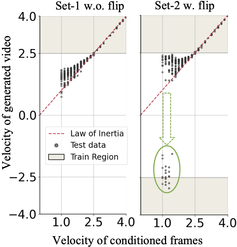
Results As shown in Figure 9, the Set-1 model generates videos with only positive velocities, biased toward the high-speed range. In contrast, the Set-2 model occasionally produces videos with negative velocities, as highlighted by the green circle. For instance, a low-speed ball moving from left to right may suddenly reverse direction after its condition frames. This could occur since the model identifies reversed training videos as the closest match for low-speed balls. This distinction between the two models suggests that the video generation model is influenced by “deceptive” examples in the training data. Rather than abstracting universal rules, the model appears to rely on memorization, and case-based imitation for OOD generalization.
We aim to investigate the ways a video model performs case matching—identifying close training examples for a given input.
Experimental Design We use uniform linear motion for this study.
Specifically, we compare four attributes, i.e., color, shape, size, and velocity, in a pairwise manner.
In other words, we build an
Through comparisons, we seek to determine the model's preference for relying on specific attributes in case matching.
Every attribute has two disjoint sets of values. For each pair of attributes, there are four types of combinations.
We use two combinations for training and the remaining two for testing.
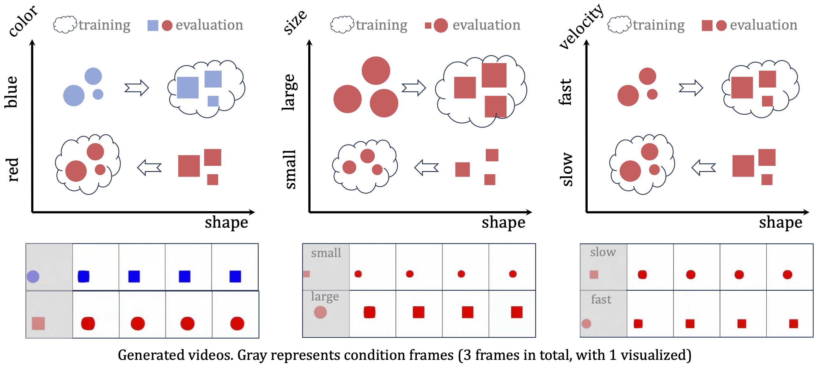
Observation 1 We first compare color, size and velocity against shape. For example, in Figure 11 (1), videos of red balls and blue squares with the same range of size and velocity are used for training. At test time, a blue ball changes shape into a square immediately after the condition frames, while a red square transforms into a ball. Similar observations can be made for the other two settings. This suggests that diffusion-based video models inherently favor other attributes over shape, which may explain why current open-set video generation models usually struggle with shape preservation.

Observation 2 The other three pairs are presented in Figure 13.
For velocity v.s. size, the combinatorial generalization performance is surprisingly good.
The model effectively maintains the initial size and velocity for most test cases beyond the training distribution.
However, a slight preference for size over velocity is noted, particularly with extreme radius and velocity values
(top left and bottom right in subfigure (1)).
In subfigure (2), color can be combined with size most of the time.
Conversely, for color v.s. velocity in subfigure (3), high-speed blue balls and low-speed red balls are used for training.
At test time, low-speed blue balls appear much faster than their conditioned velocity. No ball in the testing set changes its color,
indicating that color is prioritized over velocity.
Conclusion Based on the above analysis, we conclude that prioritization order is as
follows: color > size > velocity > shape.
What kind of data can actually enable conceptually-combinable video generation? We try to answer this question by indentifing three foundamental combinatorial patterns through experimental design.
Attribute composition As shown in Figure 9 (1)-(2), certain attribute pairs—such as velocity and size, or color and size—exhibit some degree of combinatorial generalization.
Spatial composition
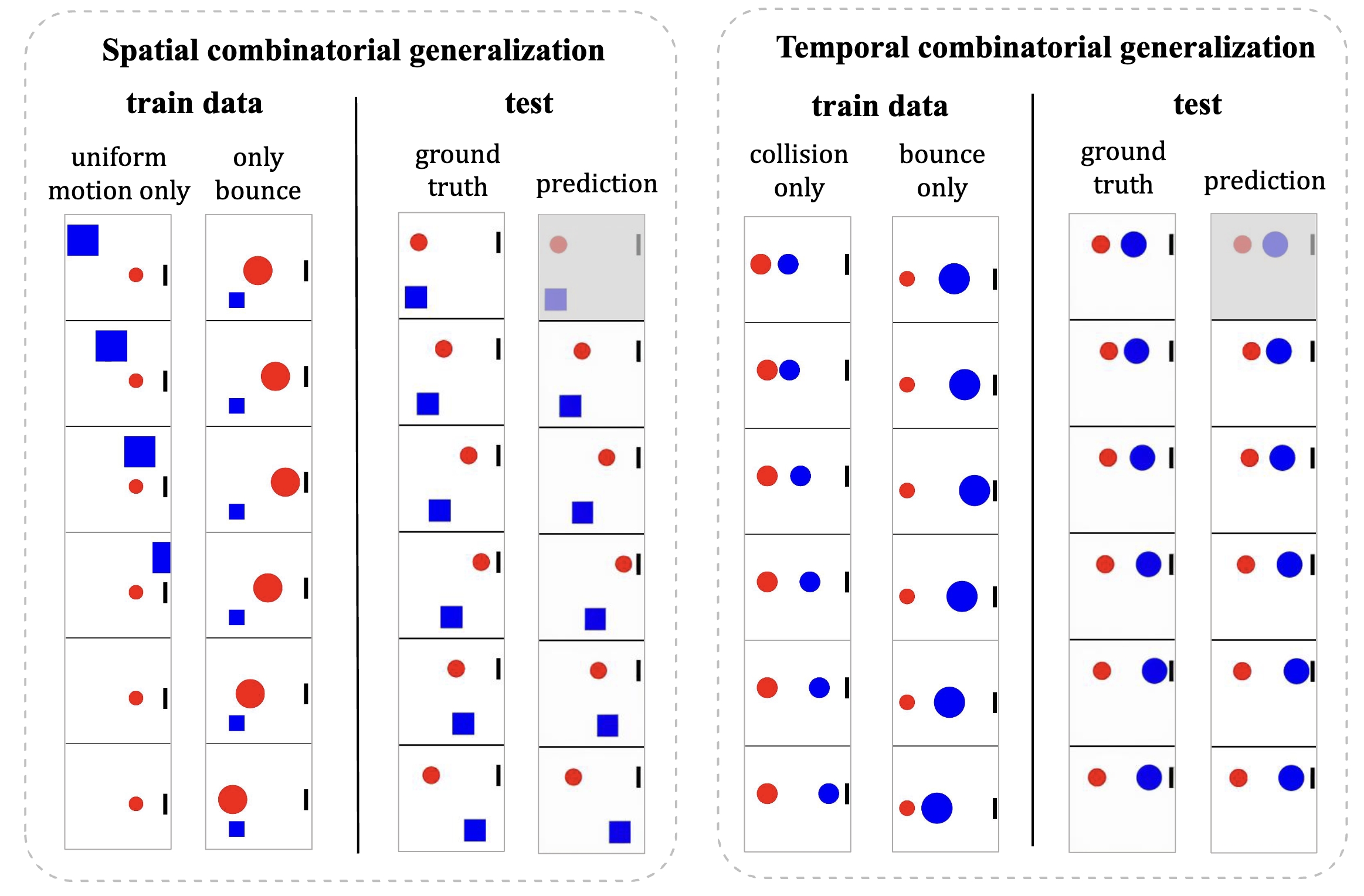
As given by Figure 14 (left side), the training data contains two distinct types of physical events.
One type involves a blue square moving horizontally with a constant velocity while a red ball remains stationary.
In contrast, the other type depicts a red ball moving toward and then bouncing off a wall while the blue square remains stationary.
At test time, when the red ball and the blue square are moving simultaneously, the learned model is able to generate the scenario ]
where the red ball bounces off the wall while the blue square continues its uniform motion.
Temporal composition
As illustrated on the right side of Figure 14 , when the training data includes distinct physical
events—half featuring two balls colliding without bouncing and the other half showing a red ball bouncing off a wall—the model learns to combine
these events temporally. Consequently, during evaluation, when the balls collide near the wall, the model accurately predicts the collision and
then determines that the blue ball will rebound off the wall with unchanged velocity.
For a video generation model to function as a world model, the visual representation must provide sufficient information for complete physics modeling. In our experiments, we found that visual ambiguity leads to significant inaccuracies in fine-grained physics modeling. For example, in Figure 16 , it is difficult to determine if a ball can pass through a gap based on vision alone when the size difference is at the pixel level, leading to visually plausible but incorrect results. Similarly, visual ambiguity in a ball’s horizontal position relative to a block can result in different outcomes. These findings suggest that relying solely on visual representations, may be inadequate for accurate physics modeling.

Experimental Setup We experimented with collision scenarios and DiT-B models, adding two variants: one conditioned on vision and numerics, and the other on vision and text. For numeric conditioning, we map the state vectors to embeddings and add the layer-wise features to video tokens. For text, we converted initial physical states into natural language descriptions, obtained text embeddings using a T5 encoder, and then add a cross-attention layer to aggregate textual representations for video tokens.
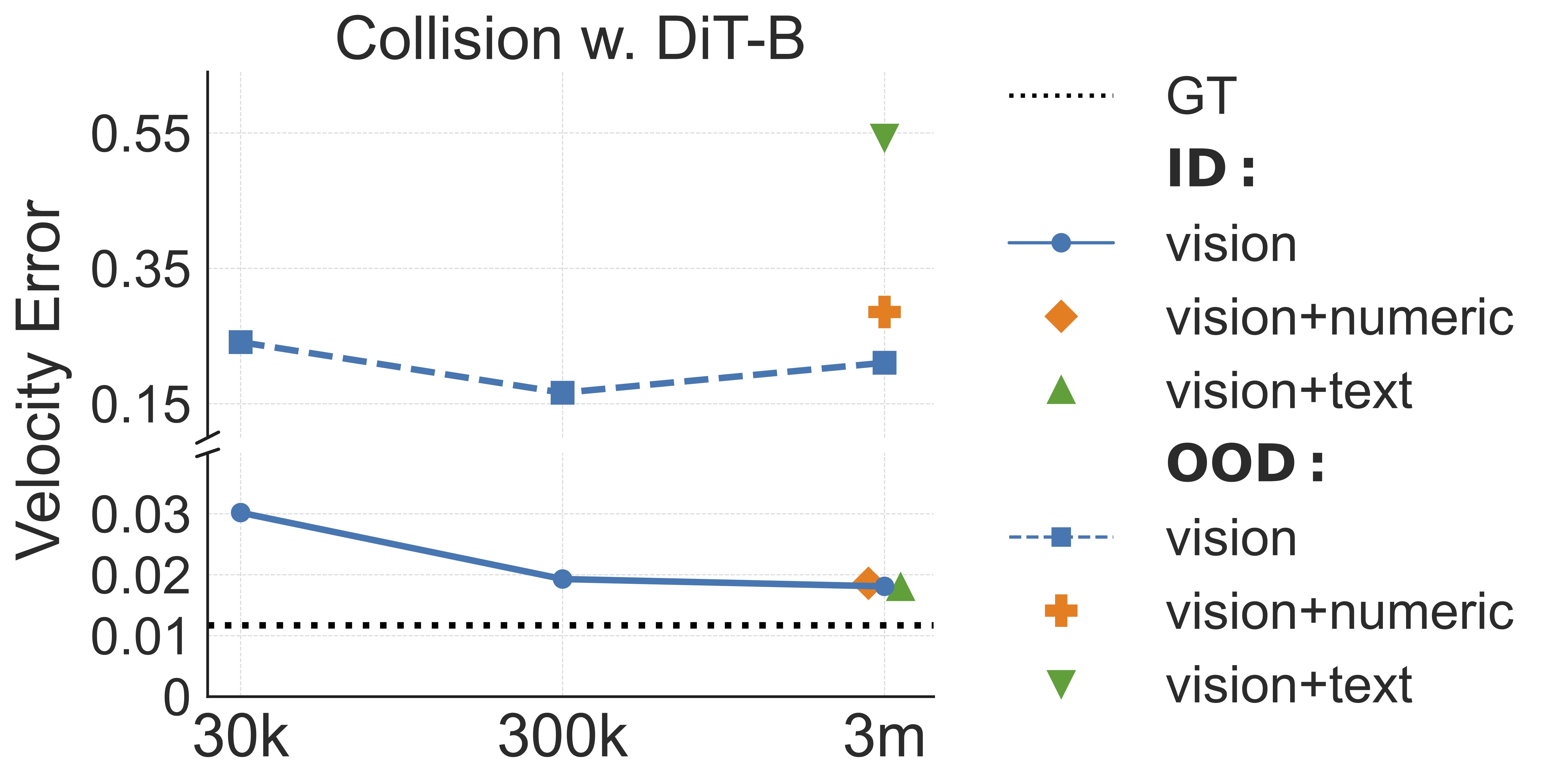
Results As shown in Figure 18, for in-distribution generalization, adding numeric and text conditions resulted in prediction errors comparable to using vision alone. However, in OOD scenarios, the vision-plus-numerics condition exhibited slightly higher errors, while the vision-plus-language condition showed significantly higher errors. This suggests that visual frames already contain sufficient information for accurate predictions, and probobaly the best modality for generalization. However, the text knowledge in our setting is limited to the problem setting. Instead, large language models are often trained with large-scale corpus containing nearly all knowledge in human history. We'd like to triger a discussion on whether this kind of knowledge can be used to make the physical law discovery problem feasible.
Our hypothesis on why the preference exists
Since the diffusion model is trained by minimizing the loss associated with predicting VAE latent, we hypothesize that the prioritization may be related to the distance in VAE latent space (though we use pixel space here for clearer illustration) between the test conditions and the training set.
Intuitively, when comparing color and shape as in Figure 11 (1), a shape change from a ball to a rectangle results in minor pixel variation, primarily at the corners. In contrast, a color change from blue to red causes a more significant pixel difference. Thus, the model tends to preserve color while allowing shape to vary.
From the perspective of pixel variation, the prioritization of color > size > velocity > shape can be explained by the extent of pixel change associated with each attribute.
Changes in color typically result in large pixel variations because it affects nearly every pixel across its surface. In contrast, changes in size modify the number of pixels but do not drastically alter the individual pixels' values. Velocity affects pixel positions over time, leading to moderate variation as the object shifts, while shape changes often involve only localized pixel adjustments, such as at edges or corners. Therefore, the model prioritizes color because it causes the most significant pixel changes, while shape changes are less impactful in terms of pixel variation.
Experimental Setup
To further validate this hypothesis, we designed a variant experiment comparing color and shape, as shown in Figure 19. In this case, we use a blue ball and a red ring.
For the ring to transform into the ball without changing color, it would need to remove the ring's external color, turning it into blank space, and then fill the internal blank space with the ball's color, resulting in significant pixel variation.
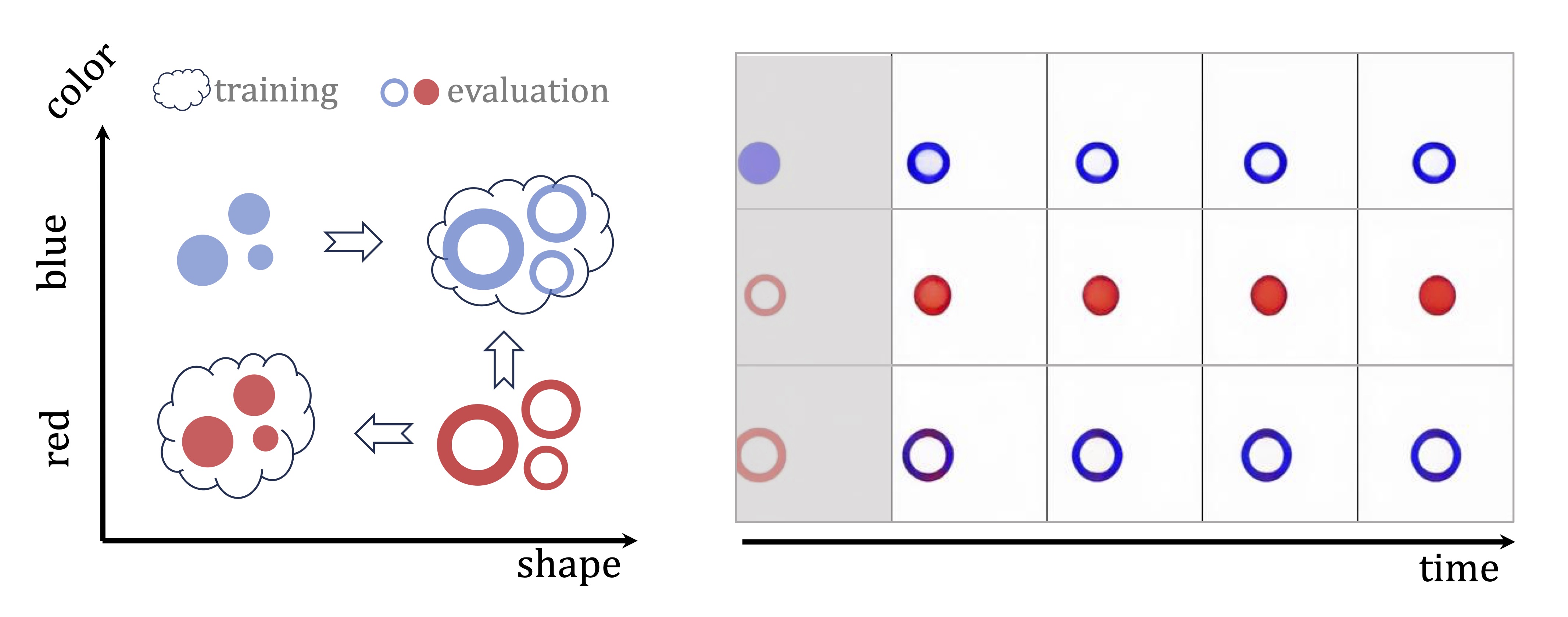
Results Interestingly, in this scenario, unlike the previous experiments shown in Figure 11 (1), the prioritization of color > shape does not hold. The red ring can transform into either a red ball or a blue ring, as demonstrated by the examples. This observation suggests that the model's prioritization may indeed depend on the complexity of the pixel transformations required for each attribute change. Future work could explore more precise measurements of these variations in pixel or VAE latent space to better understand the model's training data retrieval process.
We observe three types of generated videos in terms of how accruate the physical event is. Type 1: The generated videos are visually similar or identical to the ground-truth video from physical simulation. Type 2: The generated videos are different from ground-truth videos but human eyes feel it is reasonable (not breaking any physical laws). Type 3: A person can easily tell the video is wrong.
@article{kang2024how,
title={How Far is Video Generation from World Model? -- A Physical Law Perspective},
author={Kang, Bingyi and Yue, Yang and Lu, Rui and Lin, Zhijie and Zhao, Yang, and Wang, Kaixin and Huang, Gao and Feng, Jiashi},
journal={arXiv preprint arXiv:2411.02385},
year={2024}
}